loss_func = LaplaceNLLLoss
# Fit a linear regression using mean squared error.
regression = GaussianNet(n_feature=1, n_hidden=2, n_output=1)     # RegressionModel()
params = regression.parameters()
optimizer = torch.optim.Adam(params, lr = 0.001)

#####################
# Training
####################


my_images = []
fig, (ax1, ax2) = plt.subplots(figsize=(20,7), nrows=1, ncols=2)

# train the network
for epoch in range(4000):


    prediction, scales = regression(x)

    loss_all = loss_func(prediction, y, scales, reduction='none')     # must be (1. nn output, 2. target)
    loss = torch.mean(loss_all)
    #if t%10 == 0: print (loss)

    optimizer.zero_grad()   # clear gradients for next train
    loss.backward()         # backpropagation, compute gradients
    optimizer.step()        # apply gradients
    if np.mod(epoch, 100) == 0:
      sort_x, _ = torch.sort(x, dim=0)
      sort_prediction, sort_scales = regression(sort_x)

      print (loss)

      # plot and show learning process
      plt.cla()
      ax1.cla()
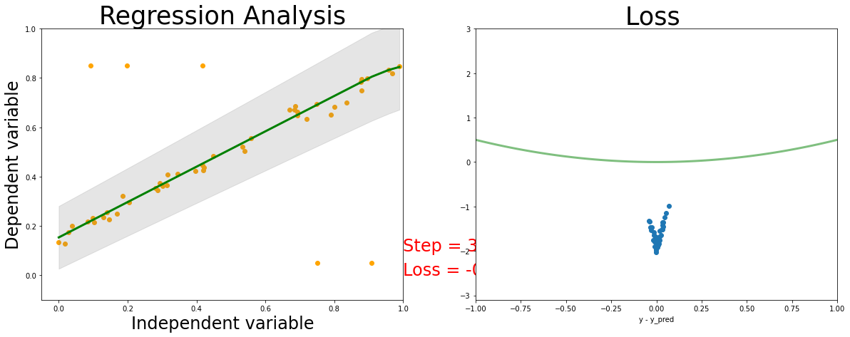
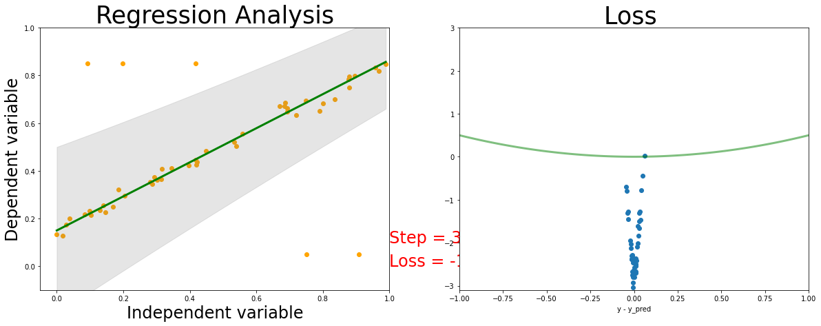
      ax1.set_title('Regression Analysis', fontsize=35)
      ax1.set_xlabel('Independent variable', fontsize=24)
      ax1.set_ylabel('Dependent variable', fontsize=24)
      ax1.set_xlim(-0.05, 1.0)
      ax1.set_ylim(-0.1, 1.0)
      ax1.scatter(x.data.numpy(), y.data.numpy(), color = "orange")
      ax1.plot(sort_x.data.numpy(), sort_prediction.data.numpy(), 'g-', lw=3)
      dyfit = 2 * sort_scales.data.numpy()  # 2*sigma ~ 95% confidence region

      ax1.fill_between( np.squeeze(sort_x.data.numpy()),
                         np.squeeze(sort_prediction.data.numpy() - dyfit),
                       np.squeeze(sort_prediction.data.numpy()  + dyfit),
                 color='gray', alpha=0.2)

      #l2_loss_plot_x = np.linspace(0,1,num=100)
      #y_plot_true = l2_loss_plot_x * scale_true + shift_true
      #ax1.plot(l2_loss_plot_x, y_plot_true, 'k')

      ax1.text(1.0, 0.1, 'Step = %d' % epoch, fontdict={'size': 24, 'color':  'red'})
      ax1.text(1.0, 0, 'Loss = %.4f' % loss.data.numpy(),
              fontdict={'size': 24, 'color':  'red'})
      diff = prediction.data.numpy() - y.data.numpy()

      ax2.cla()
      l2_loss_plot_x = np.linspace(-1,1,num=100)
      ax2.plot(l2_loss_plot_x, 0.5*l2_loss_plot_x**2, color="green", lw=3, alpha=0.5)
      ax2.scatter(diff,  loss_all.data.numpy())
      ax2.set_title('Loss ', fontsize=35)
      ax2.set_xlabel('y - y_pred')
      ax2.set_ylim(-3.1, 3)
      ax2.set_xlim(-1, 1)
      # Used to return the plot as an image array
      # (https://ndres.me/post/matplotlib-animated-gifs-easily/)
      fig.canvas.draw()       # draw the canvas, cache the renderer
      image = np.frombuffer(fig.canvas.tostring_rgb(), dtype='uint8')
      image  = image.reshape(fig.canvas.get_width_height()[::-1] + (3,))

      my_images.append(image)