Note we also compare Gaussian distribution and Laplace distirbution to empiracally find the $95%$ region with respect to their scale.

We found out 95% Confidence interval is $Gaussian ( 2 \sigma) == Laplace(3b)$

Scoring Rules for Quantile and Interval Forecasts

Interval Score

classical case of $(1 - ) % $ prediction interval
with lower and upper endpoints (predictive quatiles) at level $\alpha/2$ and $ 1 - /2$
Interval score \[ S_\alpha^{int}(l, u ;x) = (u-l) + \frac{2}{\alpha}(l-x) \mathbb{1} \{x < l\} + \frac{2}{\alpha} (x - u)\mathbb{1}\{x > u\}\]

$\alpha_1= 0.02,\alpha_2= 0.05,\alpha_3=0.1$ (implying nominal coverages of 98%,95%,90%)

import numpy as np

def interval_score(x, lower, upper, alpha=0.05):
  assert np.all(upper>=lower), "Upper should be greater or equal to lower. Please check are you giving the upper and lower in propoer order "
  return (upper - lower) + (2/alpha)*(lower-x)*(x<lower) + (2/alpha)*(x-upper)*(x>upper)

x = np.linspace(1.0, 12.0)
l = 5.0
u = 8.0
iscore = interval_score(x, l, u)

import matplotlib.pyplot as plt

plt.plot(iscore)

x = np.linspace(1.0, 12.0)
l = 5.0*np.ones_like(x)
u = 8.0*np.ones_like(x)
iscore = interval_score(x, l, u)
plt.plot(iscore)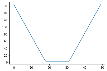

CRPS

import scipy.stats as stats
def crps_gaussian(y_pred, y_std, y_true, scaled=True):
    """
    Return the negatively oriented continuous ranked probability score for
    held out data (y_true) given predictive uncertainty with mean (y_pred)
    and standard-deviation (y_std). Each test point is given equal weight
    in the overall score over the test set.
    Negatively oriented means a smaller value is more desirable.
    """

    # Flatten
    num_pts = y_true.shape[0]
    y_pred = y_pred.reshape(
        num_pts,
    )
    y_std = y_std.reshape(
        num_pts,
    )
    y_true = y_true.reshape(
        num_pts,
    )

    # Compute crps
    y_standardized = (y_true - y_pred) / y_std
    term_1 = 1 / np.sqrt(np.pi)
    term_2 = 2 * stats.norm.pdf(y_standardized, loc=0, scale=1)
    term_3 = y_standardized * (2 * stats.norm.cdf(y_standardized, loc=0, scale=1) - 1)

    crps_list = -1 * y_std * (term_1 - term_2 - term_3)
    crps = np.sum(crps_list)

    # Potentially scale so that sum becomes mean
    if scaled:
        crps = crps / len(crps_list)

    return crps

data = np.random.normal(loc=1.0, scale=1.0, size=1000)
mus = np.ones_like(data)
sigmas = np.ones_like(data)
crps_gaussian(data, sigmas, mus, scaled=False)

587.2681356774692

PLot Gaussian and Laplace with same interval

For the laplace distribution

$f(med) = $ and therefore $D(x_{0.5}) = \frac{\sigma^2}{2n}$ confidence interval of the median

\[ x - \frac{ u_{1 - \alpha/2} (n-1)0.707 s}{\sqrt{n}} \leq median \leq x + \frac{u_{1 - \alpha/2} (n-1)0.707 s}{\sqrt{n}}\]

Example :

laplace disitrbution L(0, 2) : variance $s^2 = 2b^2 = 2.246$ Substitutint in above equation median = 0.0119 estimated b = 1.0596

mu = 0.0119
b = 1.0596
n = 50
var = 2*b**2; print ("Variance : ", var)

confidence_95 = (stats.norm.ppf(1 - 0.05/2) * 0.707 * var**0.5)
print (mu-confidence_95 , mu+confidence_95)

Variance :  2.24550432
-2.0645642208852193 2.088364220885219

stats.norm.ppf(1 - 0.05/2) * 0.707 * var

3.111583069190677

for i in np.linspace(0,0.99,num=10):
  print (i,stats.norm.ppf(i), stats.laplace.ppf(i))

0.0 -inf -inf
0.11 -1.2265281200366098 -1.5141277326297755
0.22 -0.7721932141886848 -0.8209805520698302
0.33 -0.4399131656732338 -0.4155154439616658
0.44 -0.15096921549677725 -0.12783337150988489
0.55 0.12566134685507416 0.1053605156578264
0.66 0.41246312944140495 0.3856624808119848
0.77 0.7388468491852137 0.7765287894989964
0.88 1.1749867920660904 1.4271163556401458
0.99 2.3263478740408408 3.912023005428145

(0.29 * n**0.5)/(0.707* var**0.5 * 49)

0.039501224521614836

stats.norm.ppf(1 - 0.05/2)

1.959963984540054

import matplotlib.pyplot as plt
import numpy as np
import scipy.stats as stats
import math

mu = 0
variance = 1
sigma = math.sqrt(variance)
x = np.linspace(mu - 3*sigma, mu + 3*sigma, 100)
plt.plot(x, stats.norm.pdf(x, mu, sigma))
plt.plot(x, stats.laplace.pdf(x, mu,sigma), c='r')
plt.show()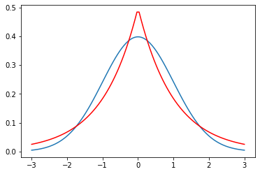

Gaussian vs Laplace

95% Confidence interval is $Gaussian ( 2 \sigma) == Laplace(3b)$

r = stats.norm.rvs(mu, sigma, size=1000)
v = ((mu - 2*sigma) < r ) & (r< (mu + 2*sigma))
np.sum(v)/1000

0.953

r = stats.laplace.rvs(mu, sigma, size=1000)
v = ((mu - 3*sigma) < r ) & (r< (mu + 3*sigma))
np.sum(v)/1000

0.952

for mu in np.linspace(0, 255, num=10):
  for sigma in np.linspace(0, 5, num=10):
    r = stats.laplace.rvs(mu, sigma, size=1000)
    v = ((mu - 3*sigma) < r ) & (r< (mu + 3*sigma))
    print (np.sum(v)/1000)

stats.laplace.ppf(1 - 0.05/2)

2.99573227355399

x = np.array([True, False])
y = np.array([True , True])
x & y

array([ True, False])

mu = 0
variance = 1
sigma = math.sqrt(variance)
b = math.sqrt(var/2)

mu + 2*sigma

2.0

mu + 3*0.67

2.0100000000000002

b = 0.67
laplace_variance = 2*b**2
print (laplace_variance)

0.8978000000000002


mu = 0
variance = 1
sigma = math.sqrt(variance)
x = np.linspace(mu - 3*sigma, mu + 3*sigma, 100)
plt.plot(x, stats.norm.pdf(x, mu, sigma))
plt.plot(x, stats.laplace.pdf(x, mu,b), c='r')
plt.show()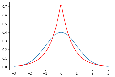

stats.laplace.ppf(0.975)

2.99573227355399

stats.laplace.ppf(0.025)

-2.995732273553991