Exponential Power Distribution

Generalized Gaussian Distirbution

Plotting the PDF and Negative log likelihood of the distribution.

Analysis on the effect of the parameters on the pdf and the nll.

import sympy.plotting as symplot
import sympy as sym
sym.init_printing(use_unicode=True)

import numpy as np
import pandas as pd
import seaborn as sns

import matplotlib.colors as mcolors
import matplotlib.pyplot as plt

color = list(mcolors.TABLEAU_COLORS)

plt.rcParams['figure.figsize'] = 25, 10 #Plot Size
plt.rcParams['legend.fontsize']=10 #Legend Size

from typing import List,Tuple

import pandas as pd
import seaborn as sns
import numpy as np

Sympy Plotting Function

def plot_exponential_power_distribution(alphas: List,
                                        betas: List,
                                        sympy_function,
                                        plot_ylim: Tuple = (0,6),
                                        plot_xlim: Tuple = (-2,2)):
    xlim = 1e-21
    
    p1 = symplot.plot(sympy_function.subs([(beta, betas[0]), (alpha, alphas[0])]), (diff,-xlim,xlim), show=False, line_color='darkgreen')
    p1[0].label = ''
    i=0
    for a in alphas:
      for b in betas:
          p = symplot.plot(sympy_function.subs([(beta,b), (alpha, a)]), (diff,-3,3), show=False, line_color=color[i%len(color)])
          p[0].label =  'beta %s, alpha %s, zero %s'% (str(b),str(a),str(sympy_function.subs([(beta,b), (diff,0),(alpha, a)])))
          p1.append(p[0])
          i = i+1

    p1.legend = True
    p1.ylim = plot_ylim
    p1.xlim = plot_xlim
    p1.show()

Probability Density function

\[ \frac{\beta}{2 \alpha \Gamma(1/\beta)} e^{- (|x - \mu | / \alpha)^{\beta}} \]

Replacing \(x - \mu\) with \(diff\) a single variable.

\[ \frac{\beta}{2 \alpha \Gamma(1/\beta)} e^{- (|diff | / \alpha)^{\beta}} \]

alpha, beta, diff = sym.symbols('alpha, beta, diff')

pdf =  ( beta / (2 * alpha * sym.gamma(1 / beta)) ) * sym.exp(-((sym.Abs(diff)/alpha)**beta))
pdf

Fixed alpha changing beta

Observtion

The Maximum is at \(beta = 2.0\) (Gaussian) at any fixed alpha
\(beta = 0.3\) the max pdf is 0.5 which is less than 1 -> can be considered for the minimum beta value

alphas = [0.1]
betas = [ 0.3, 0.4, 0.5, 1.0, 1.5, 2.0, 8.0]
plot_exponential_power_distribution(alphas, betas, pdf)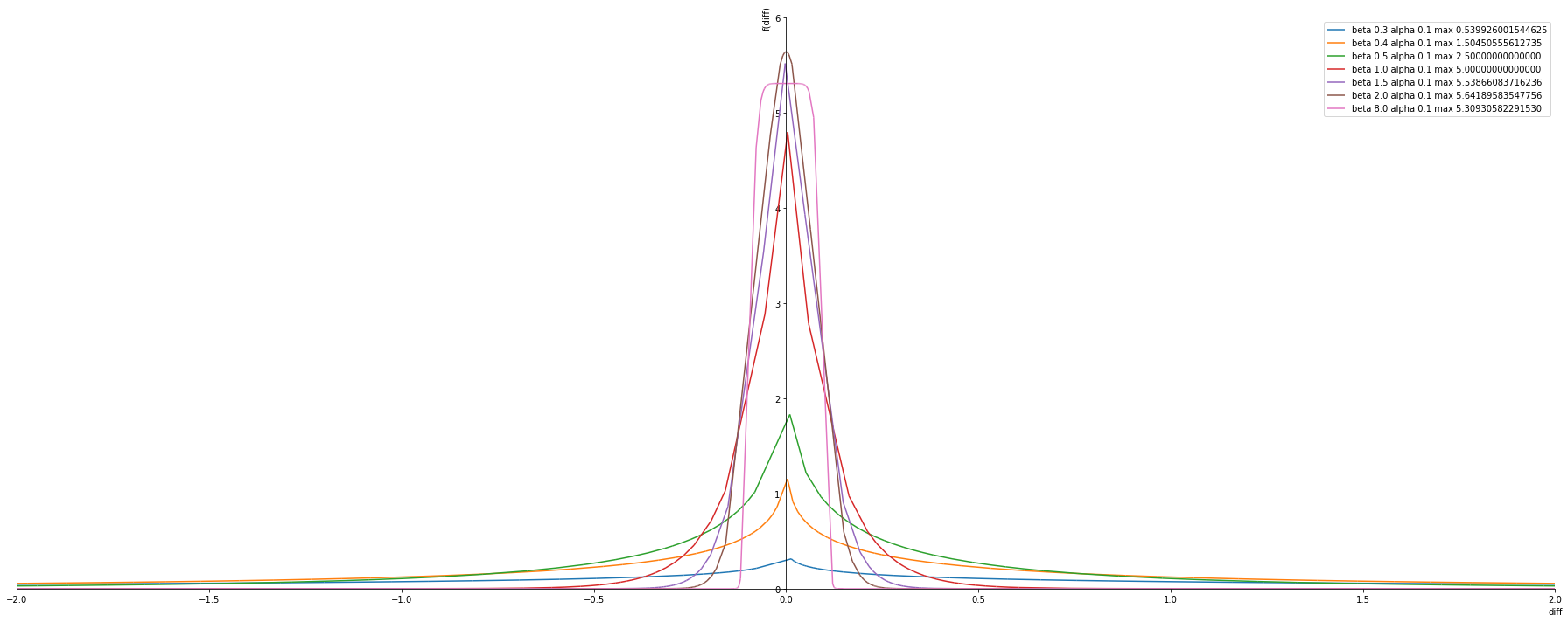

Fixed beta changing alpha

Observtion

Alpha is the variance value -> the lower the better the more confident.

alphas = [ 0.01, 0.1, 0.5, 1.0, 2.0]
betas = [ 2.0] #Gussian Distirbution
plot_exponential_power_distribution(alphas, betas, pdf)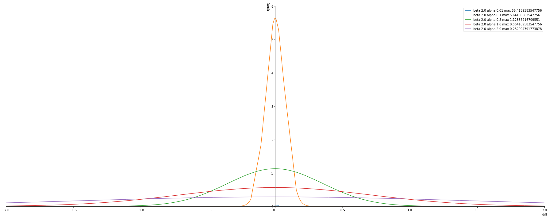

alphas = [ 0.01, 0.1, 0.5, 1.0, 2.0]
betas = [ 1.0] #Laplace distirbution
plot_exponential_power_distribution(alphas, betas, pdf)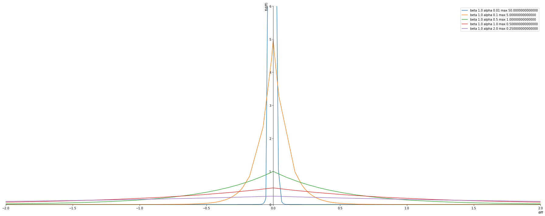

Negative log likelihood

Here we take the logarithmic of the pdf and the invert it .

The NLL are usually used as loss function in regresion problems.

nll_pdf = -1 * sym.log(pdf)
nll_pdf

nll_pdf.subs([(beta,0.5), (diff,0),(alpha, 1.0)])

alphas = [1.5, 2.0]
betas = [ 0.1, 0.5, 1.0, 2.0, 8.0]

plot_exponential_power_distribution(alphas, betas, nll_pdf, plot_ylim=(0,3))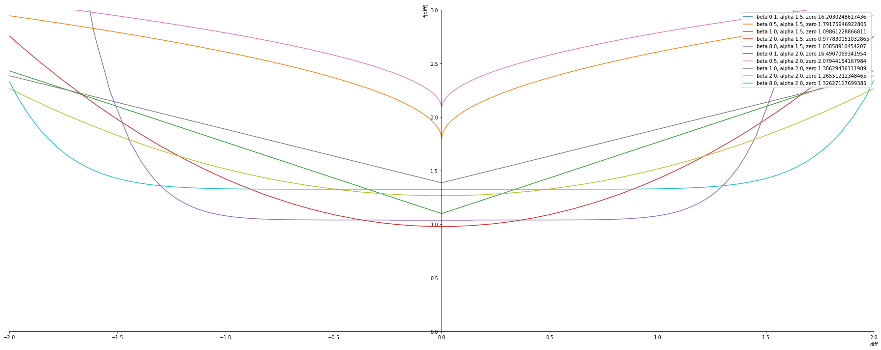

Entropy

\[ \frac{1}{\beta} - \log [ \frac{\beta}{2 \alpha \Gamma(1/\beta)}] \]

Observations

With reducing value of alpha entropy reduces (since alpha is the variance this fits perfectly)
With increasing beta the entropy reduces
- This is little counter intutive
- Expected that entropy will be low only for beta = 2 (Gaussian) since it had max value in pdf.
- But apparently when beta increases the confidence increases that the value is between some range and not a single value .

#Modelling in sympy
entropy = (1 / beta) - sym.log(beta / (2 * alpha * sym.gamma(1/beta)) )
entropy

betas = [ 0.1, 0.5, 1.0, 2.0, 8.0]
alphas = [ 0.01, 0.1, 0.5, 1.0, 2.0]

val = []
for a in alphas:
  for b in betas:
    #print ('Entropy : {}, beta: {}, alpha: {}'.format(entropy.subs([(alpha, a), (beta,b)]), b, a))
    val.append([float(entropy.subs([(alpha, a), (beta,b)])), b, a])

entropy_data_frame = pd.DataFrame(val, columns=['entropy','beta', 'alpha'])
print (entropy_data_frame.dtypes)

entropy_data_frame =  entropy_data_frame.pivot('alpha', 'beta', 'entropy')
print (entropy_data_frame.dtypes)

entropy_data_frame

entropy    float64
beta       float64
alpha      float64
dtype: object
beta
0.1    float64
0.5    float64
1.0    float64
2.0    float64
8.0    float64
dtype: object

beta	0.1	0.5	1.0	2.0	8.0
alpha
0.01	21.192390	-1.218876	-2.912023	-3.532805	-3.847046
0.10	23.494975	1.083709	-0.609438	-1.230220	-1.544461
0.50	25.104413	2.693147	1.000000	0.379218	0.064977
1.00	25.797560	3.386294	1.693147	1.072365	0.758124
2.00	26.490707	4.079442	2.386294	1.765512	1.451271

sns.heatmap(entropy_data_frame, annot=True, fmt=".1f")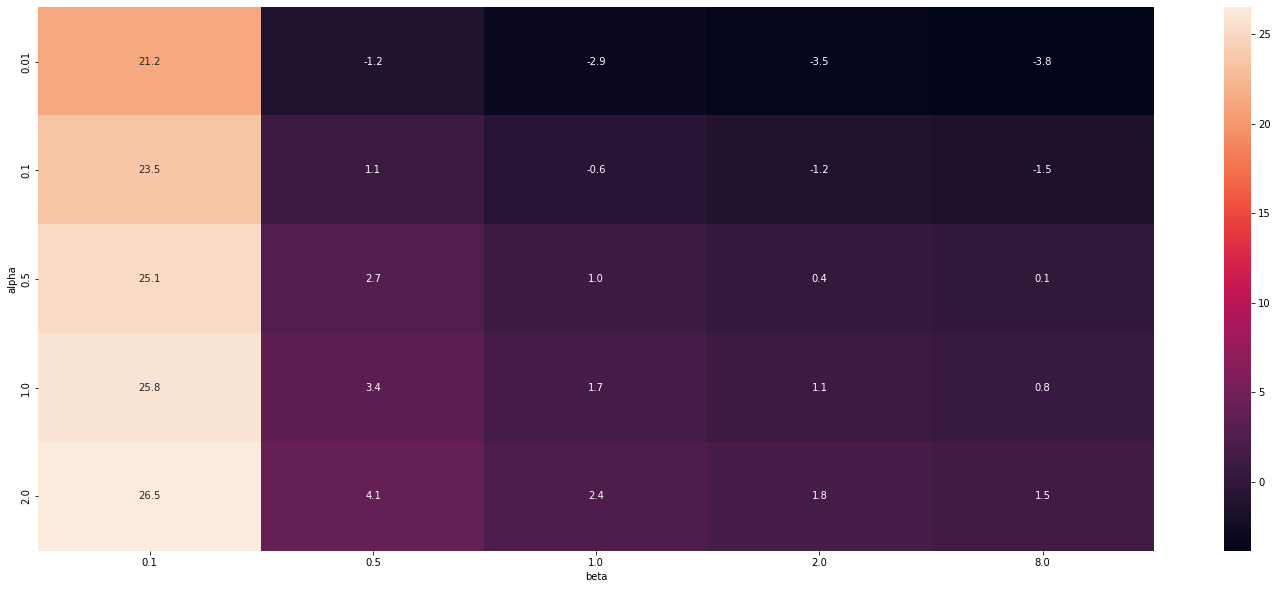

Interval

ToDO

Can we calculucalte interval from variance
Can we calculate interval from the quantile
interval is ppf function which is inverse cdf function
We have the CDF function . How to calculate the inverse CDF ?

import scipy.stats as stats

a = 0.1
b = 2.0
p = 0.9 
stats.gamma()

<scipy.stats._continuous_distns.gamma_gen at 0x7fbaf9fd26a0>

cdf = 0.5 + (sym.sign(diff)/2 )*(1/sym.gamma(1/beta))