Fibonacci Sequence: Non Recursive Formula

Plots and comparison to Exponential

In a series of Twitter posts by Matematician Tivadar Danka demonstrated the non recursive formula for the Fibonacci sequence.

I wanted to plot this equation and compare it with the exponential equation.

In the process I did some updates to the equation.

Took the absolute of the conjugate golden ratio. This helped in removing the imaginary part( (-0.6)** 1.5 = has an imaginary element)
I tried to generalize the equation and find the other forms and a equation near to exponential

golden_ratio = (1 + 5**0.5 )/2
conjugate_golden_ratio = (1 - 5**0.5 )/2

print ("Golden Ratio :", golden_ratio)
print ("Conjugate Golden Ratio :", conjugate_golden_ratio)

Golden Ratio : 1.618033988749895
Conjugate Golden Ratio : -0.6180339887498949

n = sym.symbols('n')
fibonacci = (sym.Pow(golden_ratio, n)  - sym.Pow(abs(conjugate_golden_ratio),n)) / (golden_ratio - conjugate_golden_ratio)
fibonacci

symplot.plot(fibonacci, (n,0,10), show=True, legend=True)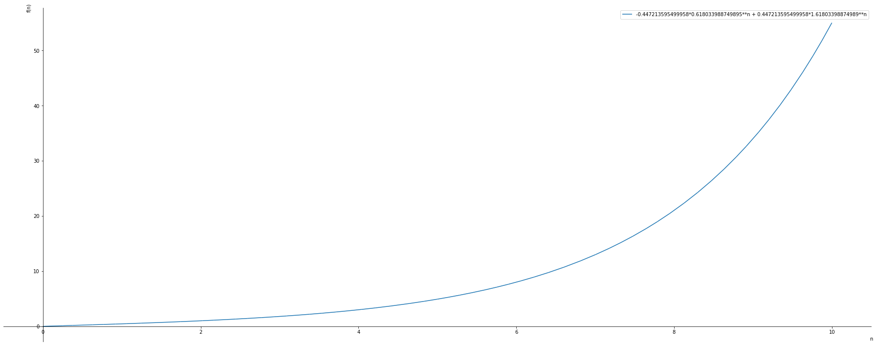

Generalizing the Fibonacci equation

We generalize the Fibonnacci equation, by parametrizing the golden ratio and the conjugate of the golden ratio.

# Generalized Fibonacci Equation

g, n = sym.symbols('g, n')

golden_ratio = (1 + g**0.5 )/2
conjugate_golden_ratio = (1 - g**0.5 )/2
fibonacci = (sym.Pow(golden_ratio, n)  - sym.Pow(abs(conjugate_golden_ratio),n)) / (golden_ratio - conjugate_golden_ratio)
fibonacci

Comparing with the exponential equation

Based on the generalized fibonacci equation, we would like to find if we can can get an approximate of the exponential equation

#symplot.plot(fibonacci.subs(g, 4), (n,0,10), show=True, line_color='darkgreen')


graphs= sym.plotting.plot(fibonacci.subs(g, 35), fibonacci.subs(g, 34),fibonacci.subs(g, 33), sym.exp(n),  (n,0,8), title="Fibonacci", legend= True, xlabel='n', ylabel='f(x)', show=False)


for i, graph in enumerate(graphs):
 graph.line_color=color[i%len(color)]

graphs.show()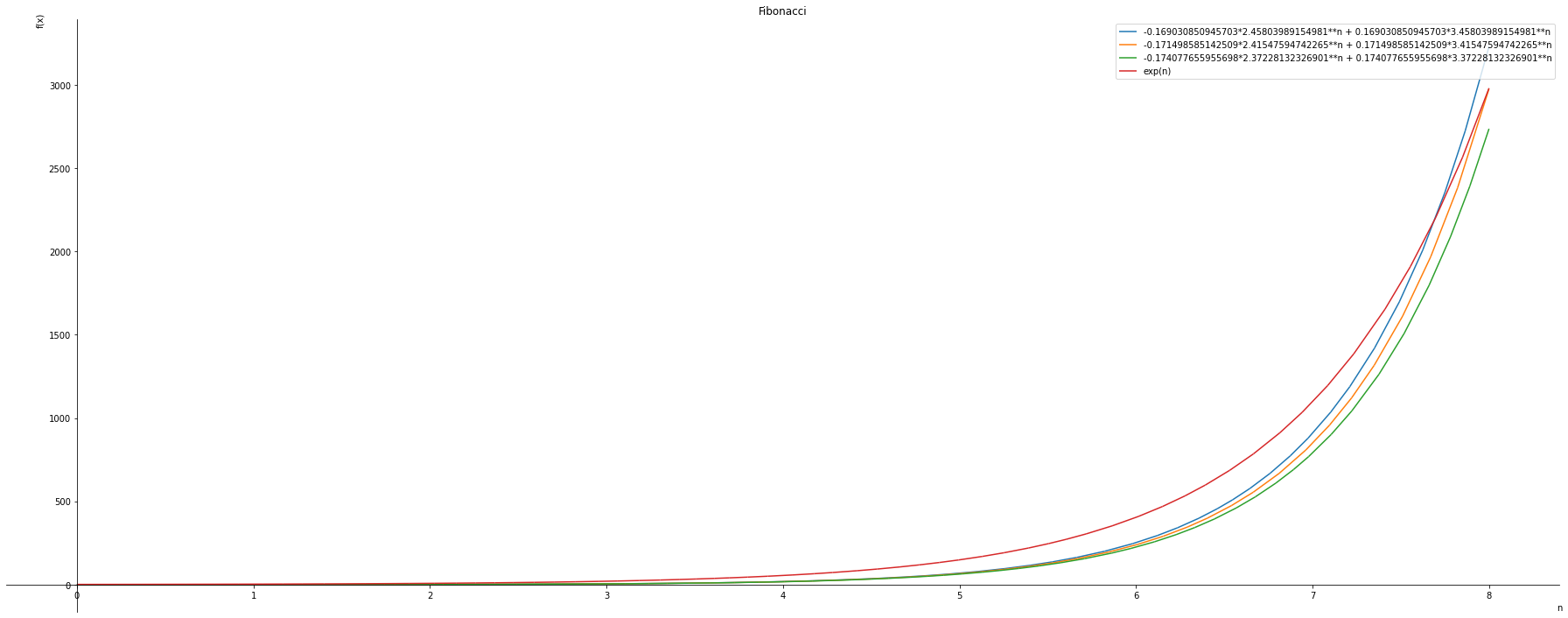

Comparing with the exponential equation (region [0 - 1])

#symplot.plot(fibonacci.subs(g, 4), (n,0,10), show=True, line_color='darkgreen')


graphs= sym.plotting.plot(fibonacci.subs(g, 35), fibonacci.subs(g, 34),fibonacci.subs(g, 33), sym.exp(n),  (n,0,1), title="Fibonacci", legend= True, xlabel='n', ylabel='f(x)', show=False)


for i, graph in enumerate(graphs):
 graph.line_color=color[i%len(color)]

graphs.show()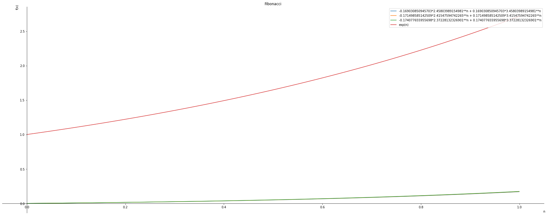

Random Ideas

Comparison with the Power equations.

\[ f(n) = constant^{n} \]

Observations

The constant if less than 1 then it inverts
If constant is 1 then the equation is flat
Higher the constant higher the slope

graphs= sym.plotting.plot(sym.exp(n), 2**n, 0.1**n,1**n,2.3**n,2.67**n,(n,0.0,1), title="Exponential", legend= True, xlabel='n', ylabel='f(x)', show=False)


for i, graph in enumerate(graphs):
 graph.line_color=color[i%len(color)]

graphs.show()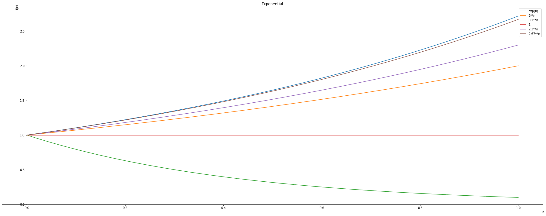

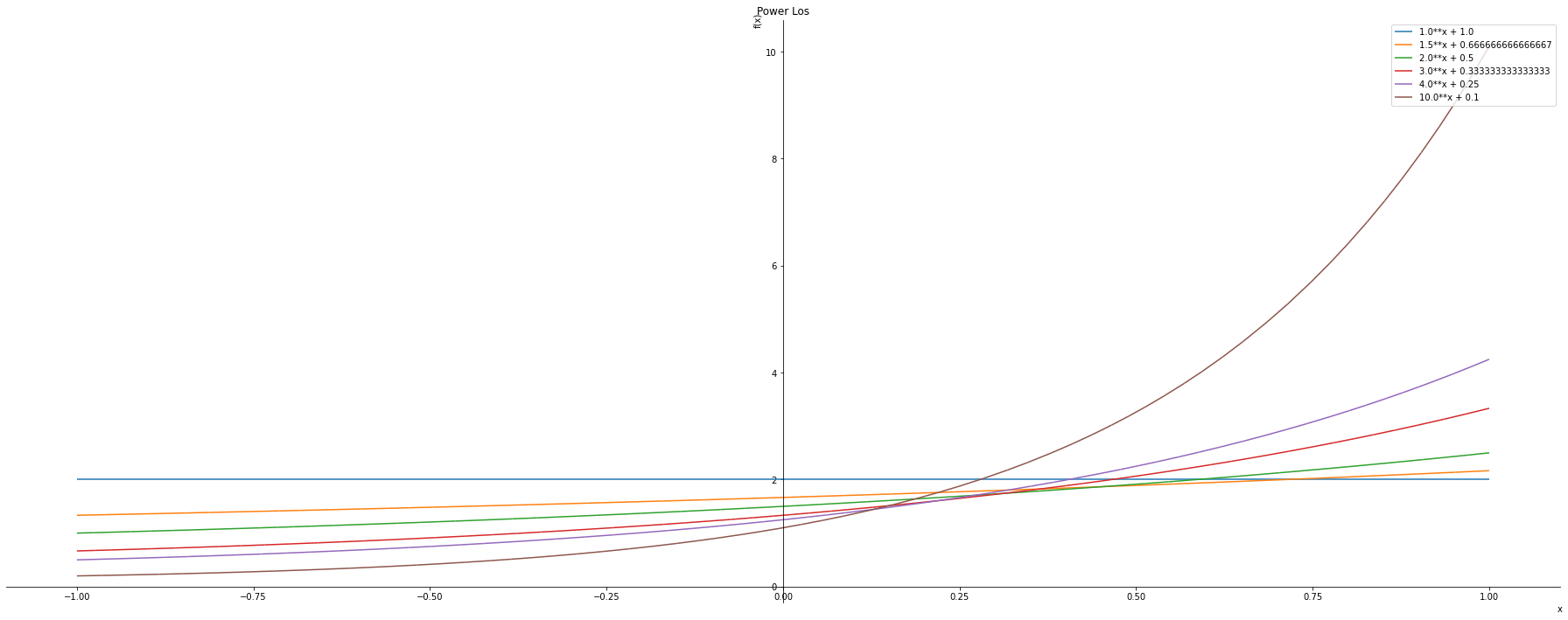
Converting the power equation to loss function

Inoder to the make the loss function, for higher slope lines the loss at zero should be lesser
so the highest slope equation should have lowest loss
This is achieved by adding the inverse of the constant to the loss

\[ f(n) = constant^{n} + \frac{1}{constant} \]

n, x = sym.symbols('n, x')
loss = n**x + 1/n 

#n hasto be grater than 1 

graphs = sym.plotting.plot(loss.subs(n,1.),
                          loss.subs(n,1.5),
                          loss.subs(n,2.),
                          loss.subs(n,3.),
                          loss.subs(n,4.),
                          loss.subs(n,10.),
                          (x,-1,1), title="Power Los", legend= True, xlabel='x', ylabel='f(x)', show=False)

for i, graph in enumerate(graphs):
 graph.line_color=color[i%len(color)]

graphs.show()